Mathematics 280C (Spring 2013)

[ Home ] [ Math Dept ] [ UPS


Contents


Course Logistics


Day-by-Day Notes


Day and Date

Topics:
Text:
Tomorrow:
Comments:

Monday May 6

Topics: Semester Review focusing on this objectives sheet
Text:
Tomorrow:
Comments:

Friday May 3

Topics: questions on divergence; divergence theorem
Text: Divergence handout
Tomorrow: Semester Review focusing on this objectives sheet
Comments: Today we reviewed flux density, divergence and gave a geometric interpretation of the Divergence Theorem. This theorem is one of the (multivariate) fundamental theorems of calculus and tells us that, provided the correct hypotheses hold and \(S \) is a closed surface (oriented outward) that encloses the solid region \(W \), then \[\iiint_{W} \vec{\nabla} \cdot \vec{F} dV = \iint_{S} \vec{F} \cdot d\vec{A}. \]

Thursday May 2

Topics: Divergence and flux density
Text: Divergence handout
Tomorrow: questions on divergence; divergence theorem
Comments: Following up on the example yesterday where we made a geometric argument to compute the flux density of a simple vector field, today we developed a general formula for flux density (also known as the divergence) of a vector field \(\vec{F}= \langle F_1, F_2, F_3 \rangle \). Specifically, we zoomed in on a small box and computed the flux density out of the box as \(\frac{\partial F_1 }{\partial x} + \frac{\partial F_2 }{\partial y} + \frac{\partial F_3 }{\partial z}. \) We then introduced the "gradient operator" \( \vec{\nabla} = \langle \frac{\partial}{\partial x},\frac{\partial}{\partial y},\frac{\partial}{\partial z} \rangle \) and introduced the notation \(\vec{\nabla} \cdot \vec{F} \) for the divergence. We finished with a simple example.

Tuesday April 30

Topics: Questions on vector surface integrals and Divergence and flux density
Text: Divergence and flux density
Tomorrow: Divergence and flux density
Comments: Today we reviewed the fact that a density function is a function whose output at a point is the limit of a ratio. Our example was an area mass density function whose output was the limit as the size of the region goes to zero of the ratio \(\frac{\Delta m}{\Delta A} \) --- the amount of mass in a small region of the point divided by the area of that region. We then defined the volume flux density function at a point P in three dimensional space as the limit of the flux of a vector field F through a small closed surface enclosing a solid divided by the volume of that solid. This flux density function is called the divergence of the vector field F at the point P. We then computed the divergence of the vector field \( \vec{F}=\langle x,y,z\rangle\) at the origin to be 3.

Tomorrow we will develop a formula that allows us to easily compute the divergence of a differentiable vector field at any point in its domain.


Monday April 29

Topics: questions on conservative fields; more on flux
Text: 16.5
Tomorrow: Divergence and flux density
Comments: Today we reviewed flux through a surface using \(\iint_S \vec{F} \cdot d \vec{A} \) and also computed a few examples. Homwork problems are in the handout vector surface integrals.

Friday April 26

Topics: questions on conservative vector fields; flux
Text: flux, also known as vector surface integrals
Tomorrow: questions on conservative fields; more on flux
Comments: Today we noted that we could use an integral to compute the "amount", or flux of a vector field through surface. In particular, we noted that the flux through an infinitesimal area element \( d \vec{A}\) is given by \(\vec{F} \cdot d \vec{A} \) so the total flux through a surface S is \[\iint_S \vec{F} \cdot d \vec{A} \].

Thursday April 25

Topics: questions on line integrals and conservative fields; fundamental theorems, independence of path, etc.
Text: 16.3
Tomorrow: questions on conservative vector fields; flux
Comments: Today we introduced various terms and notations associated with conservative vector fields. In particular, we discussed a vector field being indendent of path, conservative or having a potential function (which I also called an antigradient). We also noted that if a vector field \(\vec{F}=\langle R_1, F_2, F_3 \rangle \) is continuous on a domain that is connected, open, and simply connected, then it is conservative if and only if \( \frac{\partial F_1}{\partial y} = \frac{\partial F_2}{\partial x}, \quad \frac{\partial F_1}{\partial z} = \frac{\partial F_3}{\partial x}, \quad \frac{\partial F_2}{\partial z}=\frac{\partial F_3}{\partial y}.\) Much of this information is summarized in the handout Conservative vector fields

Tuesday April 23

Topics: questions on line integrals; conservative vector fields
Text: 16.3
Tomorrow: questions on line integrals and conservative fields; fundamental theorems, independence of path, etc.
Comments:

Today we reviewed the meaning of the line integral of a vector field along a curve (as developed in the handout on vector curve integrals), took a look at different notations for line integrals, and did one more example. We also noted that we have now studied 6 different types of integrals: single integrals of scalar functions with domains a closed interval, double integrals of scalar functions with domain a "nice" region in the plane, triple integrals of scalar functions with "nice" domains in 3-space, line integrals of scalar functions along a curve (computing totals from density functions), surface integrals of scalar functions with domain "curvy" surfaces in 3-space, and line integrals of vector fields along a curve.

We then took a quick look at an example of the fundamental theorem of line integrals. By noting that if a vector field \( \vec{F} \) is actually the gradient of a scalar field \( \vec{F}=\nabla f \), then the line integral \(\int_C \vec{F} \) depends only on the initial and final points of the curve \(C\) and not on the rest of the curve. So If \(C_1, C_2\) are two different curves with the same initial and final points, then \(\int_{C_1} \vec{F}= \int_{C_2} \vec{F}\). Tomorrow we will state this fundamental theorem carefully and explore some of its implications.


Monday April 22

Topics: questions on integrating over a surface; vector fields
Text: 16.2; vector fields
Tomorrow: questions on line integrals; conservative vector fields
Comments:

Today we looked at some images of vector fields: a wind velocity vector field plot and a more sophisticated wind flow plot. We also looked at this handout designed to help us better understand what vector fields are.

We then started discussing the idea of integrating a vector field over a curve. As with other types of integration, we can ask

Today, we addressed "What is it?" and did one example of How do we compute it? We also spent a brief time on "What does it tell us?. Tomorrow, we'll get more practice in computing and use specific results to get a better feel for what this type of integration tells us. For a preview take a look at this handout on integrating a vector field along a curve. You can wait until after class tomorrow to work on the problems from this handout and the new assignment for problems from Section 14.2.


Friday April 19

Topics: Integrating over a surface
Text: 16.4
Tomorrow: questions on integrating over a surface; vector fields
Comments:

In class, we looked at integrating over a surface. A key part of evaluating a surface integral is expressing the area element dA in terms of the coordinates chosen to describe the surface. In the simplest cases, we can use a geometric argument to deduce an expression for dA. Today we also explored a more general procedure --- a computational approach. The basic idea and some examples are on this handout. The handout also has the assigned problems for this material.

As with integrating over a curve, we follow an approach that differs somewhat from the main approach used in the text. The text approaches integrating over curves and surfaces in terms of parametrizing the curve or surface. Our approach of computing dA is a bit more general (and modern). Specifically, we think of gridding our surface by two families of curves where curves from the two families meet non-tangentially and where the differentials \(d\vec{r}=\langle dx, dy \rangle\) for every curve in each family are easy to compute. We then use \(dA =\|d\vec{A}\|= \| d\vec{r_1}\times d\vec{r_2} \| \) as our infinitesimal area element for that surface. You are welcome to read about the text's approach to integrating over a surface in Section 16.4.


Thursday April 18

Topics: questions on integrating over a curve; Infinitesmal area elements and integrating over a surface.
Text: 16.4
Tomorrow: integrating over a surface
Comments:

In class, we looked at integrating over a surface. A key part of evaluating a surface integral is expressing the area element dA in terms of the coordinates chosen to describe the surface. In the simplest cases, we can use a geometric argument to deduce an expression for dA. In other cases, we need a computational approach. The basic idea and some examples are on this handout. The handout also has the assigned problems for this material.

As with integrating over a curve, we will follow an approach that differs somewhat from the main approach used in the text. The text approaches integrating over curves and surfaces in terms of parametrizing the curve or surface. Our approach is a bit more general. You are welcome to read about the text's approach to integrating over a curve in Section 16.2 and integrating over a surface in Section 16.4.


Tuesday April 16

Topics: Questions on integration over a curve; Cross Product of Vectors
Text: 12.4
Tomorrow: questions on integrating over a curve; Infinitesmal area elements and integrating over a surface.
Comments:

We started class with a first example of integrating over a surface. As part of this, we needed to describe the surface in terms of a chosen coordinate system and then work out an expression for the area element of the surface in that coordinate system. For the first example, the surface was a sphere and we were able to use a geometric argument to deduce an expression for the area element in spherical coordinates. We will develop a more general approach for more general situations. As part of that, we will use a new tool called the cross product of two vectors.

In the latter part of class, we defined the cross product of two vectors. The cross product of \(\vec{u}\) and \(\vec{v}\) is a new vector denoted \(\vec{u}\times\vec{v}\) and defined geometrically in relationship to the parallelogram that has \(\vec{u}\) and \(\vec{v}\) as its edges. Specfically, \(\vec{u}\times\vec{v}\) is defined geometrically by these two properties:


Monday April 15

Topics: Integrating scalar functions along a curve
Text: 16.2
Tomorrow: Questions on integration over a curve; Cross Product of Vectors
Comments: Today we looked at the idea of integrating over (or along) a curve. This required that we understand the infinitesimal length element ds which is the norm of the infinitesimal vector dr.In some cases, we will add up these small contributionsds to get the total length of the curve. In other cases, we will have a length density function λ defined at each point on the curve and we will add up small contributions of the form λds to get a total (of some quantity such as charge or mass). The handout Integration over a curve has the details and also the assigned problems.

Friday April 12

Topics: Integration in cylindrical and spherical coordinates
Text: 15.4
Tomorrow: 16.2; Integrating scalar functions along a curve
Comments: Today we used a geometric analysis to deduce that the infinitesimal volume element in spherical coordinates is \(\rho^2 \sin(\phi)\). We then practiced setting up iterated triple integrals in both cylindrical and spherical coordinates. I have assigned a number of homework problems out of two handouts for you to use for practice. The first handout is copied from a different text book and is not available in electronic form. You can pick a physical copy up from me in class. The second handout is online and involves finding totals from volume density functions.

Thursday April 11

Topics: Exam 3
Text: 14.7, 14.8, applied optimization, nonuniform density, 15.1, 15.2, 15.3, 11.3, 15.4
Tomorrow:
Comments:

Tuesday April 9

Topics: review for Exam #3
Text: review for Exam #3
Tomorrow: Exam #3
Comments:

Monday April 8

Topics: questions on spherical and cylindrical coordinates; integrating triple integrals using cylindrical coordinates
Text: 15.4
Tomorrow: review for Exam #3
Comments:

Friday April 5

Topics: cylindrical and spherical coordinates
Text: 13.4
Tomorrow: questions on spherical and cylindrical coordinates; integrating triple integrals using these coordinates
Comments: Today we took a careful look at both cylindrical and spherical coordinates.

The cylindrical coordinate transformations are:

\[ \begin{eqnarray*} x & = & r \cos \theta \\ y & = & r \sin \theta \\ z & = & z \\ & & \\ x^2 +y^2 & = & r^2 \\ \frac{y}{x} & = & \tan \theta \\ z & = &z \end{eqnarray*} \]

We then noted that the graph of \(z=c \) is a plane that is parallel to the x-axis, the graph of \(r=c \) is a right circular cylinder with axis the z-axis and of radius r and the graph of \( \theta =c \) is a vertical plane that starts at the z-axis and extends in the direction of the ray making an angle of \( \theta=c\) with the positive x-axis.

We then looked at spherical coordinates whose defining transformations, where \(\rho \geq 0 \), \( 0 \leq \theta \leq 2 \pi \), and \9 0 \leq \phi \leq \pi\) are:

\[ \begin{eqnarray*} r & = & \rho \sin \phi \\ x & = & \rho \sin \phi \cos \theta \\ y & = & \rho \sin \phi \sin \theta \\ z & = & \rho \cos \phi \\ & & \\ x^2 +y^2+z^2 & =& \rho^2 \end{eqnarray*} \]

We also noted that the graph of \( \rho =c \) is a sphere centered at the origin of radius c, the graph of \(\theta = c \) is a vertical half-plane that starts at the z-axis and extends in the direction of the ray making an angle of \( \theta=c\) with the positive x-axis and the graph of \( \phi = c \) is a cone (just half of a double cone) making an angle of \( \phi \) with the positive z-axis.

Exam #3 will be on Thursday April 11. We will use the 80-minute period from 2:00-3:20. The exam objectives are in this handout.


Thursday April 4

Topics: questions on double integrals in polar coordinates; cylindrical coordinates
Text: 15.4
Tomorrow: cylindrical and spherical coordinates
Comments: Today we did more examples of double integrals using polar coordinates. We also introduced the cylindrical coordinate system which keeps the z of Cartesian coordinates but uses polar coordinates rather than x and y. We then set up a first example of evaluating a triple integral using cylindrical coordinates. In the process we noted that one way to compute the volume of a solid in three space is to triple integrate the constant function
\(f(x,y,z )=1\) over the solid. Although the result does not have the units of volume (unless the outputs of the function \(f\) are dimensionless), it does have the correct numerical value of the volume.

Exam #3 will be on Thursday April 11. We will use the 80-minute period from 2:00-3:20.


Tuesday April 2

Topics: questions on graphing in polar coordinates; double integrals in polar coordinates
Text: 11.3
Tomorrow: questions on double integrals in polar coordinates; cylindrical coordinates
Comments: We spent today doing examples of evaluating double integrals using polar coordinates. We focused on how to describe the region of integration in terms of the \( [r, \theta] \) values of the points in the region.

Exam #3 will be on Thursday April 11. We will use the 80-minute period from 2:00-3:20.


Monday April 1

Topics: questions on polar coordinates; graphing in polar coordinates
Text: 11.3
Tomorrow: questions on graphing in polar coordinates; double integrals in polar coordinates
Comments:

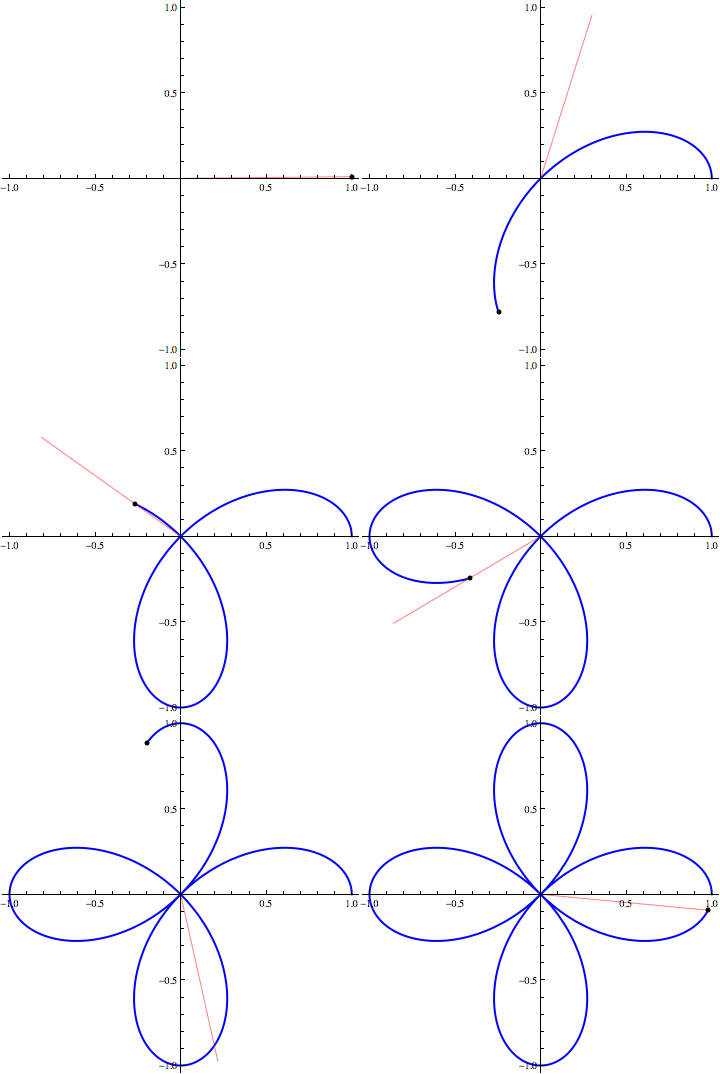
Today, we discussed the basics of polar coordinates and plotting polar curves. The animation below shows the curve r=cos(2θ) being traced out as θ increases. Notice how the r values are negagive for some angles.

Tomorrow, we'll use our ability to graph polar equations to evaluate double integrals over regions that are best described in the polar coordinate system. polar curve animation

Exam #3 will be on Thursday April 11. We will use the 80-minute period from 2:00-3:20.


Friday March 29

Topics: questions on triple integrals; polar coordinates
Text: 11.3
Tomorrow: questions on polar coordinates; graphing in polar coordinates
Comments: Today we introduced polar coordinates (in two dimensions). These coordinates are useful when the sets and functions we are using have an inherent "circular" nature. The polar coordinate transformations are: \[ \begin{eqnarray*} x & = & r \cos \theta \\ y & = & r \sin \theta \\ & & \\ x^2 +y^2 & = & r^2 \\ \frac{y}{x} & = & \tan \theta \end{eqnarray*} \]

Exam #3 will be on Thursday April 11. We will use the 80-minute period from 2:00-3:20.


Thursday March 28

Topics: questions on double integrals; triple integrals
Text: 15.3
Tomorrow: questions on triple integrals; polar coordinates
Comments:

Today, we looked at examples of triple integrals and the corresponding iterated integrals in three variables. A triple integral involves adding up infinitely many infinitesimal contributions to a total over a solid region of space. To describe this type of region, we need a three-dimensional coordinate system so we end up with an iterated integral in three variables (that is, the three coordinate variables). For the examples we looked at today, we used cartesian coordinates. In some other example, we might find it convenient to use some other coordinate system. This week, we will look at polar coordinates in two dimensions and two other coordinate systems for three dimensions: cylindrical coordinates and spherical coordinates.

Exam #3 will be on Thursday April 11. We will use the 80-minute period from 2:00-3:20.


Tuesday March 26

Topics: questions on double integrals and area density problems; triple integrals
Text: 15.3
Tomorrow: questions on double integrals; triple integrals
Comments: Today we focused on setting up double integrals where the domain of integration was a set of the form \( \{(x,y): a \leq x \leq b, f(x) \leq y \leq g(x) \} \) or \( \{(x,y): a \leq y \leq b, p(y) \leq x \leq q(y) \} \). We also used and example of computing a total charge on a plate by double integrating an area charge density function for the plate.

At the end of the hour we introduced the concept of triple integrals over solid regions in three space. This idea is a natural extension of the use of double integrals and is supported by a version of Fubini's Theorem that is phrased in terms of functions on three variables.


Monday March 25

Topics: questions on double integrals over rectangles; double integrals over general regions
Text: 15.2; area density handout
Tomorrow: questions on double integrals and area density problems; triple integrals
Comments: Today we quickly reviewed Fubini's theorem which is the result allowing us to easily compute double integrals by iterating regular integrals rather than by taking the limit of Riemann sums. We then went through a few examples of setting up a double integral and then converting it into an iterated integral when the domain of the function is not a rectangle. We will be doing much more of this in the near future.

I also passed out two new Handouts. The Introduction to Density handout gives the basics of what a density function really is and has a few straightforward exercises involving constant density functions. It also has a "reading" exercise designed to help show how often density functions are used even though they might not be referred to as density functions. In this light, if \( f(x,y) \geq 0 \) at every point \( (x,y) \) in the region R, then the double integral you can think of the double integral \[\iint\limits_{R}f(x,y) \ dA \] can be thought of in two different ways depending on the units that are assigned to f(x,y)

The second Handout was on Area Density Problems and provides some example problems whose solution requires that you use a double integral to find the total accumulation of various area density functions over various regions.

  1. as the volume of the solid that lies above the region R in the xy-plane and below the graph of z=f(x,y) and
  2. as the total accumulation of a distance area density function f(x,y) over the region R.

Friday March 15

Topics: questions on nonuniform density; double integrals
Text: 15.1
Tomorrow: questions on double integrals over rectangles; double integrals over general regions; area density
Comments: We went over the geometric intuition of finding volumes using double integrals, reviewed Riemann sums of functions on two variables and introduced the notation for double integrals and iterated double integrals. We also stated the important Fubini's theorem for double integrals

Fubini's Theorem: If \(f(x,y)\) is continuous at all points in a rectangle R of all points (x,y) with \(a \leq x \leq b \mbox{ and } c\leq y\leq d\) except for the points on a finite set of curves of area zero, then \[\iint\limits_{R}f(x,y) \ dA = \int_a^b \left(\int_c^d f(x,y) dy \right) \ dx =\int_c^d \left(\int_a^b f(x,y)\ dx \right) \ dy.\] We then worked two examples.


Thursday March 14

Topics: questions on lagrange multipliers; Nonuniform Density Handout
Text: Nonuniform Density Handout
Tomorrow: questions on nonuniform density; double integrals
Comments: We used another example to work through the set up for Lagrange multipliers. Then we reviewed basic properties of density functions. Specifically, a linear mass density function \( \lambda(x) \) outputs the limit as \(\delta x \) goes to zero of the ratio \( \frac{\delta m}{\delta x} \) of the mass \(\delta m ) of a line segment of length \(\delta x \). The total mass of a linear object with linear mass density function \( f(x) \) is then the integral \(\int \lambda(x) dx\). Linear charge densities are computed in a similar fashion. We then looked at an example how to represent a linear charge density function on a line segment and used our representation to compute the total charge.

We ended the hour by seeing how we can extend the ideas of Riemann sums to finding the volumes of solids under the graph of a function on two variables \(z=f(x,y) \).


Tuesday March 12

Topics: questions on Lagrange multipliers; more on Lagrange multipliers
Text: 14.8
Tomorrow: questions on lagrange multipliers; Nonuniform Density Handout
Comments: We worked through several examples of constrained optimization using Lagrange multipliers.

Monday March 11

Topics: questions on constrained optimization; Lagrange multipliers
Text: 14.8
Tomorrow: questions on Lagrange multipliers; more on Lagrange multipliers
Comments: We worked through a constrained optimization problem following the method that involves solving the constraint equation for one variable and substituing it into the objective function. Doing this turned our example into an optimization of a continuous function on a closed bounded domain so we were guaranteed a global maximum value (and global minimum value).

We then used a sequence of slides to outline a second approach to constrained optimization --- the method of Lagrange multipliers. The underlying intuition of this approach is that a minimizer or maximizer of a constrained problem will occur at a "first" or "last" point where level sets of the objective function meet the constrained domain. We then tracked the gradient fields of the constrained functions level sets and the level sets of the objective function and noted that the minimizers and maximizers occurred at points where these gradients are parallel. Thus, the method for using Lagrange multipliers to solve \[\begin{eqnarray*} \mbox{Maximize: } w & = & f(x,y,z) \\ \mbox{Subj. to: } C & = & g(x,y,z) \end{eqnarray*}\] is to find all points \((x,y,z)\) and all numbers \( \lambda \) that solve the system of equations \[\begin{eqnarray*} \nabla f(x,y,z) & = & \lambda \nabla g(x,y,z) \\ g(x,y,z) & = & C \end{eqnarray*}\]


Friday March 8

Topics: constrained optimization; 14.7
Text: 14.7
Tomorrow: questions on constrained optimization; Lagrange multipliers
Comments: We reviewed Taylor polynomials on one variable and how they are used to justify the Second Derivative Test for functions on one variable.

We also set up the algebra for showing that a purely quadratic function on two variables \(z=Ax^2 +2Bxy +cy^2 \) can be rewritten in a form recognizable as related to elliptic paraboloids \( z= \frac{1}{A} \left[ (Ax+By)^2 +(AC-B^2)y^2 \right]\). In this form we can see that depending on the signs of \( A\) (or \(C\)) and \( AC-B^2 \), the quadratic is the equation of a paraboloid vertexed at \( (0,0) \) (opening up or down depending on the sign of \(A\) or a parabolic hyperboloid (with saddle point at \((0,0) ) \).

Returning to Taylor polynomials on two variables, we saw that that the second derivative test for functions on two variables comes directly from evaluating the second order Taylor polynomial associated with the function \(f(x,y) \) at a critical point where the gradient is the zero vector. Comparing this polynomial with our rewritten quadratic function on two variables leads directly to the Second Derivative Test for functions on two variables.

We then finished the class period by looking at constrained optimization problems. These are problems where we seek to maximize (or minimize) an objective function \(f(x,y) \) or \(f(x,y,z) \) subject to one or more constraint equations. We worked through most of the first problem on this handout just before the end of class.


Thursday March 7

Topics: Exam #2
Text:
Tomorrow: constrained optimization; 14.7
Comments:

Tuesday March 5

Topics: questions on extreme values, review for Exam #2
Text: Exam Review
Tomorrow: Exam #2
Comments:

Monday March 4

Topics: questions on differentials and extreme values; more on extreme values
Text: 14.7
Tomorrow: questions on extreme values, review for Exam #2
Comments: We worked through a careful example of finding an absolute maximum (and minimum) when given a continuous function on a closed bounded domain. This included checking the boundary components as well as finding all possible critical points (which must be interior points). Here is a handout with the details of that problem.

Friday March 1

Topics: questions on differentials; extreme values
Text: 14.7
Tomorrow: questions on differentials and extreme values; more on extreme values
Comments:Today we introduced the basic vocabulary for finding extrema of functions on more than one variable. Specifically, minimizers and maximizers are inputs for the function at which a local maximum or minimum value occurs. We then verified the theorem that gives a complete list of the types of points that can be maximizers or minimizers:
We ended the hour by finding the possible minimizers and maximizers of a simple function (whose graph is a paraboloid) and noting that the only possible minimizer was the vertex of the paraboloid and hence was actually a global minimizer.

Exam #2 will be on Thursday March 7. I will supply a list of exam objectives either at the end of this week or over the weekend. Here is the Exam #2 objectives handout.

Thursday February 28

Topics: differentials; extreme values
Text: differentials (not from text); 14.7
Tomorrow: questions on differentials; extreme values
Comments: We took a quick look at what differentiability means by first reviewing the idea for functions of one variable and then thinking about how this generalizes to functions of two variables. Geometrically, we will think of a function of two variable as being differentiable at a point if zooming in on the graph of the function for that point results in a plane. This is a tangent plane. Here is a handout that outlines our in-class discussion of differentiability. We then recast these ideas in terms of linearization. The linearization of a function f is a linear function L built using information about f at a specific point (x0,y0). If the function is differentiable at a point, then the linearization based at that point is the best linear approximation. There are many contexts in which one trades in the full accuracy of a function for the simplicity of the linearization. In making this trade, it is often essential to have some handle on how much error is introduced by trading in for the linearization. We did not look into these error bounds but I include an example in this handout. Notice how the bound on the error depends on the size of the second derivatives. This makes sense geometrically since second derivatives measure how fast the rate of change of a function is changing. Intuitively, they are keeping track of how "curvy" a graph is. So, the better you know how "curvy" a graph is near a point, the better you can estimate how well a flat plane approximates the graph.

We then used a handout to look at how to use differentials to relate (infinitesimally) small changes among variables. Generally, we start with a nonlinear relation among various variables and we then compute a linear relation among the differentials for those variables. Differentials can be thought of as coordinates in the "zoomed-in world". Differentials are always related linearly. Ratios of differentials give rates of change. No limit is needed since the limit process has already been taken care of in "zooming in" process.

For reference, here's an applet that allows you to look at tangent planes for the graph of a function of two variables.

Exam #2 will be on Thursday March 7. I will supply a list of exam objectives either at the end of this week or over the weekend.


Tuesday February 26

Topics: questions on directional derivatives; differentials; linear approxmations
Text: 14.5; differentials problems handout
Tomorrow: questions on differentials ; differentials; extreme values
Comments: Today we explored how gradients can be used to find vectors normal to a surface with equation \(f(x,y,z)=c\) at a point P. In particular, we think of the equation as giving us a level surface for the function \(f(x,y,z)\) so that \(\nabla f_P\) is a vector orthogonal (and hence normal) to the level surface of \(f\) that contains P.

We also recalled the fact that differentiability for functions on one variable, \(f(x)\), at a point \(P= x_0\) means that the "zoomed in" portion of the graph of the function near P is indistinguishable from a line -- the tangent line to \(f\) at \(x_0\). The linearization of the function at the point \(x_0\) is the related function \(L(x)= f(x_0)+f'(x_0)(x-x_0)\). We then extended this idea to functions on two variables, \(f(x,y)\), and noted that the two dimensional analog of differentiability is that the "zoomed in" portion of the graph of \(z=f(x,y)\) near a point \((x_0,y_0) \) will be indistinguishable to a plane -- the tangent plane of \(f\) at the point \((x_0,y_0) \). Although the existence of both partial derivatives at a point is not sufficient to guarantee a tangent plane (i.e., differentiability), we noted that a function will be differentiable at \((x_0,y_0) \) if there is an open set containing \((x_0,y_0) \) for which the partial derivatives of \(f\) exist at every point in that open set. In this case, the linearization of the function \(f\) at \((x_0,y_0) \) is the related function \(L(x,y)=f(x_0,y_0)+f_x(x_0,y_0)(x-x_0)+f_y(x_0,y_0)(y-y_0)\). The graph \(z=L(x,y)\) is the tangent plane to \(f\) at \((x_0,y_0)\).

I then passed out a handout designed to help you see that differentiable functions have gradients at every point in their domain and that we can use level sets to draw enough gradients to have a very good understanding of how a function on two variables behaves. Tomorrow, we will focus on differentials and how to use them in a more modern way than is stressed in the textbook.

Here is a link to the results of the midcourse survey. Comments are paraphrased and in boldface font. Obvious results are: five people want more in-class examples; one person does not find the computer generated graphics useful; one person does not find the topics/text/tomorrow or daily notes information useful. Two comments (each from only one person) worth discussion are: have longer due dates for homework and laughter can be a bit disruptive.

Exam #2 will be on Thursday March 7. I will supply a list of exam objectives either at the end of this week or over the weekend.


Monday February 25

Topics: questions on gradients and directional derivatives; differentials and tangent planes
Text: 14.4
Tomorrow: questions on directional derivatives; differentials; linear approxmations
Comments: We started by reviewing the definition and properties of the gradient vector to a function f at a point P. The gradient \(\nabla f_P \)

We also noted that the gradient operator satisfies the sum, product, and quotient rules that we know work for derivatives on a single variable.

We then reviewed the geometric interpretation and the analytic computation formulas of the directional derivative of a function f at a point P and in the direction of a unit vector u. We finished by noting that the limit definition in the textbook matches our intuition that the ' directional derivative is computing the rate of change of the function along a "slice" of the surface obtained by slicing through P in the direction of u.


Friday February 22

Topics: questions on gradients; gradients and directional derivatives
Text: 14.5
Tomorrow: questions on gradients and directional derivatives; differentials and tangent planes
Comments: In class, we continued discussing greatest rate of change. In particular, we

While the reasoning we went through to connect these two things may initially be challenging (especially dealing with the \(\vec{Bob} \) vector), the take-away messages are simple:


Thursday February 21

Topics: questions on arc length; greatest rate of change of functions
Text: 14.5
Tomorrow: questions on gradients; gradients and directional derivatives
Comments: There were a number of questions about the homework today. In particular, we saw that there can be more than one way to parametrize a curve but that the arc length of the curve does not depend on how the curve is parametrized. We also noted that algebra continues to be a very useful tool when evaluating integrals.

We then began a discussion about how one might estimate the greatest rate of change of a function on two variables at a particular point. We used carefully labeled slides showing level sets of a temperature function and conjectured that the direction of greatest rate of change of temperature at a point was orthogonal to the level set passing through that point. We also noted that, if a scale for the units of temperature (the outputs of the function) was provided along with a distance scale for the inputs, then we could estimate the magnitude of the greatest rate of change of the function at the given point. Tomorrow we will look at how to derive a formula that we can use to compute this direction and magnitude of the greatest rate of change. I also passed out a handout associated with the slides but one page was missing. Here is a copy of the full handout.


Tuesday February 19

Topics: questions on vector-valued functions; arclength of paths
Text: 12.3
Tomorrow: questions on arc length; greatest rate of change of functions
Comments: We introduced the concept of an infinitesimal displacement \( d\vec{r}= dx \hat\imath+ dy\,\hat\jmath+ dz\,\hat k \) and an infinitesimal length \( ds = \|d\vec{r}\|=\sqrt{dx^2 + dy^2 + dz^2} \) associated with a parametrized curve (also known as a parametrized path or a vector-valued function). We used these infinitesimal elements to develop the formula giving the length of a parametrized curve \(L= \int_a^b ds \)

Monday February 18

Topics: questions on planes; vector functions; derivatives of vector functions
Text: 13.1; 13.2 (vector-valued functions)
Tomorrow: questions on vector-valued functions; arclength of paths
Comments: At the beginning of class we reviewed the homework problem showing that the if one side of a triangle is a diameter of a circle and if the third point is on the circle, then the triangle is a right triangle. Most everyone used properties of dot products to solve this problem but, if you did not, please see me so that you learn how to use the properties of vectors and dot products to approach problems of this type.

We then began discussing vector-output functions: that is, functions whose inputs are real numbers but whose outputs are vectors. These functions are also called parametrized curves. We looked at examples that parametrized the unit circle and a circular helix (the slinky). The latter was \[ \vec{r}(t)=\cos(t)\,\hat\imath+ \sin(t)\,\hat\jmath+ t\,\hat k. \]

We then defined the limit of vector-valued functions and noted that \[\lim_{x\rightarrow a} \langle x(t),y(t),z(t) \rangle = \langle \lim_{x\rightarrow a} x(t),\lim_{x\rightarrow a} y(t),\lim_{x\rightarrow a} z(t) \rangle. \] From this, continuity and differentiability of vector-valued functions easily followed. In particular, we can compute derivatives of such functions "by components".

Tomorrow we will look at the physical and geometric meaning of the derivatives of vector-output functions, derive the formula for computing the length of the curve produced by a parametrized path, and introduce one of the most important concepts we will use for the rest of the semester: the length volume element \(d\vec{r}. \)


Friday February 15

Topics: questions on dot products; more on the dot product; equations of planes revisited
Text: second handout on equations of planes
Tomorrow: questions on planes; vector functions; derivatives of vector functions
Comments: Today we talked about how to use geometric arrow vectors to represent the centroid of a triangle (with vertices A,B,C) and then we used the algebra of vectors to show that the centroid was the tip of the vector, (where O is the origin of our coordinate system) \[\frac{1}{3}\vec{OA}+\frac{1}{3}\vec{OB}+\frac{1}{3}\vec{OC}.\]

Next, we reviewed the component, \(\vec{u} \cdot \vec{e}_{\vec{v}} \) of \( \vec{u} \) in the direction of \(\vec{v}\) and the projection, \( (\vec{u} \cdot \vec{e}_{\vec{v}})\vec{e}_{\vec{v}} \) of the vector \(\vec{u} \) along \(\vec{v} \).

We ended the hour by deriving the "point-normal" form for the equation of a plane \[\vec{n} \cdot \vec{P_0 P}=0\] where \(P_0, P, \vec{n}\) are, respectively, a fixed point on the plane, a variable point on the plane, and a normal vector to the plane. After two examples, we noted that if we have the equation of a plane in standard form \(ax+by+cz+d=0,\) then we can just "read off" the components of a normal vector \(\langle a, b, c \rangle\). Our last example tied together the two topics of the day (projections and point-normal forms for planar equations) by finding the distance between two parallel planes by projecting the vector between a point on one plane and a point on the other onto the common normal vector.


Thursday February 14

Topics: more on the dot product; equations of planes revisited
Text: 12.3
Tomorrow: questions on dot products; more on equations of planes.
Comments: We talked more about inner products today. First we foucssed on using our geometric understanding of vectors to determine a vector notation for the midpoint of a line segment. We then rephrased this in terms of a coordinate system to actually find the coordinates of the midpoint. It was then easy to extend the process to find the points 1/3, 3/4 or 9/10 along a segment. We then stated the primary algebraic properties of the dot product and carefully proved one to show how useful components can be. We ended the day by first introducing the notation \(\vec{e}_{\vec{v}}\) which represents the unit vector in the direction of the nonzero vector \(\vec{v} \) and then deriving the formulas for the component, \(\vec{u} \cdot \vec{e}_{\vec{v}} \) of \(\vec{u} \) in the direction of \vec{v} and the projection, \( (\vec{u} \cdot \vec{e}_{\vec{v}})\vec{e}_{\vec{v}} \) of the vector \(\vec{u} \) along \(\vec{v} \).

Tuesday February 12

Topics: using both the geometric and algebraic forms of vectors; dot product
Text: 12.3
Tomorrow: more on the dot product; equations of planes revisited
Comments: Today we began by seeing how useful both the geometric and algebraic ways of representing vectors can be. As specific examples, we found the coordinates of the midpoint of the line segment in \(R^3\) between points \(P_0(x_0,y_0,z_0 \) and \(P_1(x_1,y_1,z_1 \) by, first, using geometric position vector \(\vec{OP_0}\) geometrically added to \( \frac{1}{2}\vec{P_0P_1}\) to see that the position vector representing the sum has the midpoint of the segment at its tip. We then converted to algebraic representations of the vectors to compute that the midpoint is \(M(\frac{x_0+x_1}{2},\frac{y_0+y_1}{2},\frac{y_0+y_1}{2}). \)

As a second example, we developed the vector method of describing the points on a line L. Specifically, If \(P_0 \) is a point on line L and \(\vec{d} \) is a vector in the direction of L, then the position vector \(\vec{OP}\) for an arbitrary point \(P(x,y,z) \) on the line can be written \(\vec{OP}=\vec{OP_0}+\vec{d}\) which has a particularly nice form when written using components (see page 673 of the text).

We then finished the hour by finding a formula for the angle between two geometric vectors based at the same point and using it to define the dot product of two vectors. The geometric and component formulas for the dot product of \( \vec{u} = \langle u_1,u_2,u_3 \rangle\) \mbox{ and } \vec{v}=\langle v_1,v_2,v_3 \rangle \) are \( \vec{u} \cdot \vec{v} =\| \vec{u} \| |\vec{v} \| \cos({\theta})=u_1v_1+u_2v_2+u_3v_3\). Using the first form it is easy to see that two non-zero vectors are orthogonal precisely when their dot product is 0 and that checking whether two vectors are orthogonal is easy if we use the second form.


Monday February 11

Topics: questions on the chain rule; vectors
Text: 12.1, 12.2
Tomorrow: questions on vectors; the dot product (12.3)
Comments: We started today by introducing vectors from a geometric point of view. In this context, a vector has two defining properties: magnitude and direction. We can represent a vector in \(R^2\) by drawing an arrow whose length represents the magnitude of the vector and whose direction is indicated by the direction of the arrow. Any other arrow with the same length and direction also represents the same vector. We then defined addition, subtraction and scaling of these geometric vectors. In particular, adding vectors using arrows is accomplished by putting the base of the second arrow at the tip of the first and then drawing the arrow that starts from the base of the first and ends at the base of the second.

We then moved to a more algebraic way of representing vectors by choosing a coordinate system and noting that, if we put the base of an arrow representing a given vector, \(\vec{u} \) at the origin (this arrow is called the position vector), then the tip of the vector specifies a unique point \(P(a,b,c) \). We then introduced the notation \(\vec{u} = \langle a,b,c\rangle \) where \(a,b,c\) are called the components of the vector \vec{u}\).

We ended the hour by defining addition and scalar multiplication of vectors (both are done "by components") and computing some examples.


Friday February 8

Topics: partial derivatives; chain rule for multivariate functions
Text: 14.3; 14.6
Tomorrow: questions on the chain rule; vectors
Comments: We reviewed the notation for higher-order derivatives (second derivatives, third derivatives, etc.) and introduced the chain rule(s) for multivariate functions. Diagrams organizing the way the primary variable depends on intermediate variables and how those intermediate variables depend on the independent variables (or each other) are very useful.

Tomorrow we will begin looking at vectors.


Thursday February 7

Topics:
Text: Exam #1
Tomorrow: partial derivatives; chain rule for multivariate functions
Comments:

Tuesday February 5

Topics: Review for exam #1
Text:
Tomorrow:
Comments:

Monday February 4

Topics: questions on 14.1 and 14.2; partial derivatives
Text: 14.3
Tomorrow: Review for Exam #1
Comments: Today we noted that the limit definition of the partial derivative of a function f(x,y) with respect to y is an exact analog to the limit definition of a function on one variable. This makes computations fairly easy since we just "think of" holding the x variable constant. We also introduced two different notations for partial derivatives and how those notations look when looking at second partial derivatives. In short, the partial derivative of f(x,y,z) with respect to x at the point \(( x_0,y_0,z_0) \) is written by either \[f_x( x_0,y_0,z_0) \mathbf{\quad or \quad} \left.\frac{\partial f}{\partial x}\right|_{( x_0,y_0,z_0)} \]

Friday February 1

Topics: questions on multivariable functions; 14.2
Text: 14.2
Tomorrow: questions on 14.1 and 14.2; partial derivatives
Comments: After discussing some of the material from section 14.1, we looked at the definitions of a number of terms associated with functions on two (and three) variables. For subsets of \(\mathbf{R}^2\) we looked at examples of: interior point, boundary point, open set, closed set, boundary of a set, bounded set and unbounded set. We also briefly discussed how all of these definitions have analogs for subsets of \(\mathbf{R}^3\) and also analogs for subsets of \(\mathbf{R}^1=\mathbf{R}\).

We then reviewed the intuition that the mathematical claim \[\lim_{x\rightarrow a}f(x)=L\] means that, regardless of how x "approaches" a (either from the left or the right), the outputs f(x) are approaching the number L.

In a similar fashion, the intuitive meaning of \[ \lim_{(x,y) \rightarrow (a,b)}f(x)=L\] is: regardless of how (x,y) "approaches" (a,b), the outputs f(x,y) are approaching the number L. The big difference is that there are infinitely many ways for (x,y) to "approach" (a,b). On the other hand, there is a relatively easy way to show that a limit \(\lim_{(x,y) \rightarrow (a,b)}f(x) \) fails to exist. If we can show that there are two different paths of approach to (a,b) that yield different values, then the limit does not exist.

The first exam will be on Thursday February 7. If possible, it will be scheduled for the 80 minute period 2:00-3:20 PM. Please send me an email as to whether or not this works for your schedule as soon as possible.


Thursday January 31

Topics: questions on quadric surfaces; multivariable functions; limits
Text: 14.1; 14.2
Tomorrow: questions on multivariable functions; limits of multivariable functions
Comments: Today we introduced functions on more than one variable. Such functions are depicted by \(f:D \rightarrow C\) where D, the domain of f is a subset of \(\mathbf{R^2}\) and C, the codomain of f is a set containing all of the outputs of f.

We also talked about using traces (slices of the graph that are parallel to the coordinate planes) to improve graphs of functions on two variables. We then talked about how every z-trace corresponds to a level set in the xy-plane and that these level sets can help us to understand the outputs of the function f even if we don't have a three-dimensional graph.

Tomorrow we will say a bit more about level sets for functions on three variables, introduce terminology describing open and closed sets in higher dimensions and begin talking about limits of multivariable functions.

Click on the following link to see an image giving level curves of temperature over North America. Level curves of temperature

The first exam will be on Thursday February 7. If possible, it will be scheduled for the 80 minute period 2:00-3:20 PM. Please send me an email as to whether or not this works for your schedule as soon as possible.


Tuesday January 29

Topics: questions on quadric surfaces; more graphing of quadric surfaces; introduction to multivariable functions
Text: 12.6; 14.1
Tomorrow: questions on quadric surfaces; multivariable functions; limits
Comments: We finished graphing quadric surface examples today (hyperboloids of two sheets, elliptical paraboloids and hyperbolic paraboloids). In doing so we focused on using traces (curves on the surfaces obtained by slicing the surface with planes parallel to the coordinate planes). We also started talking about functions on several variables (only two variables today) and noted that such a function would be one whose values are the temperature of a planar object at the various points in the domain plane. such a function would be written \(z=T(x,y) \). On Thursday we will start the process of understanding both the geometry of this type of function as well as how to apply the ideas of calculus to them.

The first exam will be on Thursday February 7. If possible, it will be scheduled for the 80 minute period 2:00-3:20 PM. Please send me an email as to whether or not this works for your schedule as soon as possible.


Monday January 28

Topics: cylinders and quadric surfaces
Text: 12.6
Tomorrow: questions on quadric surfaces; more graphing of quadric surfaces; introduction to multivariable functions
Comments: Today we started talking about cylinders and quadric surfaces. We spent some time making it clear that not all cylinders are the "right circular cylinders" from our past experience. We also noted that if the line used you build a cylinder (by tracing out a planar curve) is parallel to a coordinate axis, then that variable does not occur in the equation of the cylinder. We also illustrated how to graph surfaces in 3-D by carefully sketching an ellipsoid and less carefully sketching a cone and a hyperboloid of one sheet. Tuesday we will finish talking about quadric surfaces and introduce how to use traces and level sets to obtain geometric information about multivariable functions.

The first exam will be on Thursday February 7. If possible, it will be scheduled for the 80 minute period 2:00-3:20 PM. Please send me an email as to whether or not this works for your schedule as soon as possible.


Friday January 25

Topics: questions on equations of planes handout
Text: 11.5; conic sections
Tomorrow: 12.6; cylinders and quadric surfaces
Comments:

In discussing planes today we noted that it is possible to use algebra to determine the equation of a plane if we know three non-collinear points on that plane. This is in sharp contrast to the geometrically motivated methods we developed using the slopes \(m_x^z, m_y^z\).

In class, we also reviewed some basics of ellipses, parabolas, and hyperbolas. In particular, we started from a purely geometric definition for each type of curve and used a coordinate system to get an analytic description. In all three cases, the analytic description is a quadratic equation in two variables. Since they are in the book, we skipped many of the details of how the analytic descriptions follow from the geometric. As a small challenge, you can fill in the steps that we skipped over between the geometric definition and the most common form of an analytic descriptions.

We can also turn this around and ask about the graph of any quadratic equation in two variables. It is a fact that the graph of any quadratic equation in two variables is an ellipse, a parabola, or a hyperbola (or a degenerate case). That is, the graph of any equation of the form \[ Ax^2+2Bxy+Cy^2+Dx+Ey+F=0\qquad A,B,C\textrm{ not all zero} \] is an ellipse, a parabola, or a hyperbola. It can be shown that you can determine which type of curve by computing \(AC-B^2\). If this quantity is positive, the graph is an ellipse. If this quantity is zero and one of D or E is nonzero, the graph is a parabola. If this quantity is negative, the graph is a hyperbola.

Tomorrow, we move to three-dimensions so we will be dealing with quadratic equations in three variables and the corresponding graphs that are surfaces in space.


Thursday January 24

Topics: questions on problems from Section 12.2 and the 3D handout, spheres, cylinders and other surfaces in space; planes (part 1)
Text: equations of planes handout
Tomorrow:11.5; conic sections
Comments:

Today we worked on gaining geometric insight into planes and their equations. In particular, in computing, say, \(m_x\), it doesn't matter where we "slice" the plane as long as we hold \(y\) constant.

I will often include mathematics symbols on this page and will be using MathJax to do so. Please let me know if the following looks like the quadratic formula to you. If not, please tell me which browser you are using. \[ x= -b \pm \frac{\sqrt{b^2-4ac}}{2a} \]


Tuesday January 22

Topics: Course information sheet, functions of more than one variable; points, lines, distance and spheres in space
Text:12.2
Tomorrow: questions on problems from Section 12.2, spheres, cylinders and other surfaces in space; planes (part 1)
Comments:
Today we covered the basics of a 3-dimensional cartesian coordinate system and discussed the equations of spheres and planes. Equations of spheres come directly from the distance formula and equations of planes that are parallel to one of the coordinate planes (the \(xy\)-plane, \(yz\)-plane and \(xz\)-plane) have equations of the form \(z=c_1, x=c_2, y=c_3\), respectively, where \(c_1, c_2, c_3\) are constants.

You should read the portions of Section 12.2 that deal with spheres and right circular cylinders and start work on the homework on the 3D Basics handout


Handouts


Exam Objectives


Generally Useful Links


Writing and Studying Tips


Examination Archive

[Exam 1: Fall 2012___] [Exam 2: Fall 2012___] [Exam 3: Fall 2012___] [Exam 4: Fall 2012___]

[Exam 1: Spring 2008] [Exam 2: Spring 2008] [Exam 3: Spring 2008] [Exam 4: Spring 2008] [Exam 5 with Final: Spring 2008]